Cosmolological Implications of Weakly Interacting Massive Particles

by John Terning

A report submitted for the course
PHY 3400:  Selected Topics in Physics,
in conformity with the requirements
for the degree of

Master of Science

 at the
University of Toronto
Department of Physics
October, 1985

1. Introduction

In recent years, particle physicists have become increasingly interested in the use of cosmological calculations as tests for their hypotheses about elementary particles. Not only did particles in the early Universe have energies that far exceed the limits of present day accelerators, but also, densities at these times were so large that even weakly interacting particles like neutrinos possessed mean free paths shorter than 3 x 10^8 m. Under these conditions, particles that interact with normal matter only weakly or gravitationally can produce significant effects, whose repercusions could still be measurable at the present time.

Constraints from Cosmology can usually be obtained by asking the question: could a Universe containing a certain type of particle evolve into the Universe that we presently observe? In this paper we will find mass--lifetime constraints on particles whose strongest interaction is the weak interaction, and mass--coupling constant constraints on particles that interact with normal matter only gravitationally, by requiring that their present energy density not exceed the critical energy density, and that density perturbations in the early Universe be allowed to grow into galaxies.

(Warning! The equations have not been completely converted to html yet, proceed with caution.)

2. Stable Weakly Interacting Massive Particles

At the present time, observable galaxies appear to be engaged in a rapid expansion; so it would seem that in the past the matter of the Universe was more densely packed than it is now. For the galactic matter to have escaped the gravitational potential well of this denser era, it must have been much more energetic. If we continue to trace this behaviour back further and further in time, we come to more densely packed epochs, with even more energetic particles; and eventually we come to a singularity^1 where all particles are ultra- relativistic. This is the essence of Big Bang Cosmology.

The point that will prove to be central to our discussion of stable^2 weakly interacting massive particles (WIMPs^3) is that these particles were once moving ultra-relativistically, and were so densely packed that reactions occurred very quickly, and hence, at very early times all particles comprised a relativistic gas in thermal equilibrium. This runs counter to the usual cases in thermodynamics where thermal equilibriums are established after some period of time; but in the case of Cosmology, the Universe rapidly goes into a thermal equilibrium which is eventually destroyed. This being the case, we can treat different particles in the early Universe in a manner somewhat analogous to, say, the different modes of vibration and rotation of atoms, or to different radation modes inside a reflecting cavity.

To begin a discussion of particles in the early Universe, it is helpful to recall some results from Cosmology which are derived using the Robertson-Walker metric^4. Most importantly, distances between fundamental points (i.e. points following the expansion of space-time) grow in time proportionally to a scale factor R(t). Since, by the de Broglie relation, momenta are inversely proportional to wavelengths, they decrease with time. More concretely, if a particle has a momentum p_1 at time t_1 , at any subsequent time t, the particles momentum is

p(t) = p_1 R(t_1)/R(t) . (2.1)

For ultra-relativistic particles, this decrease in energy is often referred to as "red- shifting away." From this relation it is obvious that the energy of a relativistic gas, and hence its temperature, will decrease as the Universe expands. More precisely, since kT , where k is Boltzmann's constant and T is the temperature, is a measure of the average energy of a particle in thermal equilibrium, the temperature of an ultra-relativistic gas is given by

T(t) = constant/R(t) . (2.2)

We are now in a position to ask what happens to neutral massive spin 1/2 particles as the universe expands, and the relativistic gas it contains cools. When the temperature^5 is much larger than the mass, m_x of a particle X, the two competing processes of creation and annihilation are held in balance: X particles annihilate with anti-X particles, but other particles in the gas have sufficient energy to create more X's when they annihilate or decay^6. For any reaction that destroys X's, there is a reversed reaction that creates X's, and these two types of reactions occur, on average, equally often. During this period the number of X particles per comoving volume^35 is constant, however, as the temperature falls below m_x, particles which have sufficient energy to produce X's become increasingly rare, in accordance with the Boltzmann factor exp(-m_x/kT). Thus, although X's continue to annihilate, their rate of production decreases rapidly with decreasing temperature, and so the number of X particles per comoving volume declines. The annihilation of X particles does not continue unabated though, since the annihilation rate is proportional to the X number density, n, times the anti-X number density, which is assumed^7 to be equal to n, so as n decreases, the annihilation rate decreases like n^2. For this reason, the decrease in n due to annihilation eventually becomes insignificant in comparison to the decrease in n due to the general expansion of the Universe. Qualitatively, it becomes harder and harder for the X's to find anti-X's to annihilate with, and so they eventually behave as if no annihilation is allowed. Mathematically the rate of change of n was expressed by Lee and Weinberg [3] as

d n/dt = - 3 ( Rdot(t)/R(t)) n(t) - < sigmav> n^2(t) + < sigmav> neq^2(t) , (2.3)

where < sigmav> is the thermal average of the X anti-X annihilation cross section times the relative velocity, and neq is the number density of X particles in thermal equilibrium; that is

neq(T) = 2 /(2pi)^3 int_0^infinity 4 pi p^2 dp (exp(( p^2 + m_1^2)^(1/2) /kT ) + 1)^-1 (2.4)

where the factor 2 comes from assuming X has two spin states (and hbar = c = 1, as throughout).

It can be shown that in a Universe with a flat^8 Robertson-Walker metric the Hubble parameter is

H = Rdot/R = (8 pi rho G/3 )^(1/2) , (2.5)

where G is the gravitational constant, and rho is the energy density of the relativistic gas^9:

rho = N_f a T4 = N_f ( pi^2/15) (kT)^4 . (2.6)

N_f here is the effective number of degrees of freedom,

N_f = (1/2) ( n_b + 7/8 N_f ) (2.7)

where n_b and N_f are the total number of internal degrees of freedom^10 for all bosons and fermions present in equilibrium in the gas.

When the temperature is below m_x, the velocities of the X particles are non- relativistic; for Dirac particles this means that the annihilation cross section in the center of mass frame is proportional to 1/v, therefore < sigmav> is velocity, and hence temperature independent^11. If X interacts only weakly, and m_x « M_z, the Z boson mass, we can write < sigmav> as

< sigmav> = ( G_F^2/2pi) m_x^2 N_A , (2.8)

where N_A is a dimensionless factor which takes into account the various channels the annihilation can proceed into^12. Unfortunately eq. (2.8) is not valid for large m_x; this can be rectified by noting the correspondence evident in the GSW electroweak theory^13:

G_F/2^(1/2) --> g^2/(8((4m_x^2 - M_z^2 )^2 + M_z^2 Gamma_z^2) cos^2 theta_w ) , (2.9)

and

e = g sin theta_w . (2.10)

So,

< sigmav> = e^4 m_x^2 N_A /(64 pi((4m_x^2 - M_z^2 )^2 + M_z^2 Gamma_z^2)cos^4theta_w sin^4theta_w) , (2.11)

where theta_w is the Weinberg angle, and Gamma_z is the resonance width of the Z boson. We are making the approximation here that all the X particles have the same energy, m_x; if we took into account the distribution of energies, the peak in the cross section at m_x = M_z would be lowered and spread out.

We are now ready to attempt a calculation of the number density of X particles that survive to the present time. Eq. (2.3) can be simplified by making the substitution

n = f T^3 , neq = f_eq T^3 . (2.12)

Using eq. (2.2), this removes the explicit cosmic expansion dependence from the equation, giving

d f /dt = < sigmav> (45/8 pi^3 N_f k^4G)^(1/2) (f^2 - f_eq^2) . (2.13)

Rewriting the temperature as

x = k T/ m_x (2.14)

yields

d f/dx = b (f^2 - f_eq^2) (2.15)

where

b = < sigmav> (m_x/k^3) (45/8 pi^3 N_f G)^(1/2) . (2.16)

The boundary condition for eq. (2.15) is that as x --> infinity , f(x) approaches f_eq(x), which, from eq. (2.4), is given by

f_eq(x) = k^3/(2 pi^2) int_0^infinity du u^2 (exp (u^2 + x^-2)^(1/2) + 1)^-1) . (2.17)

It is expected the number of particles per comoving^35 volume, which is proportional to f, remains approximately equal to the number of particles per comoving volume in equilibrium, f_eq, until the chemical equilibrium is destroyed at the freezing temperature. The number density of X particles in equilibrium is determined by the temperature, and decreases rapidly as T falls below m_x, but the total number density of X particles can only be reduced by expansion and annihilation (which decreases rapidly with n). The freeze-out, occurs when the rate of change of n due to the cosmic expansion, -3H n, becomes much larger than the rate of change of n due to annihilation, < sigmav> n^2. This condition is roughly equivalent to requiring that the mean free time of the X particles becomes greater than the characteristic expansion time. In terms of our new variables, Lee and Weinberg [3] defined the freezing temperature, T_f, by

d f_eq/dx = b f_eq^2 , at x_f = k T_f / m_x . (2.18)

Below the freezing temperature, f becomes much larger than f_eq, (see fig. 1) so eq. (2.15) can be approximated by

d f/dx = b f^2 , x < x_f . (2.19)

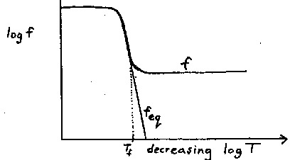
Fig. 1. Sketch of behaviour of f = n T^3 and f_eq = neq T^3. See ref. [3].

If the approximation is made that particles are non-relativistic for temperatures below their mass, then eq. (2.17) can be simplified:

f_eq(x) approx k^3/pi^2 int_0^infinity du u^2 (exp (x u^2/2 + 1/x) + 1)^-1 (2.20a)

approx k^3/pi^2 exp(-1/x) int_0^infinity du u^2 exp(-xu^2/2 ) , T « m_x (2.20b)

approx 2k^3 exp(-1/x)/(2 pi x)^(3/2) (2.20c)

Thus eq. (2.18) becomes

exp (1/x_f) (x_f^(-1/2) - 3 x_f^(1/2) /2) = 2 b k^3/(2 pi)^(3/2) (2.21)

which can be solved numerically to determine x_f. Whenx_f « 2/3 we have

f(x_f) approx f_eq(x_f) approx 1/(b x_f^2) . (2.22)

Now, solving eq. (2.19) yields

f(x) = 1/(b x_f^2 + b (x_f - x) ) . (2.23)

For m_x ť 2 _1 10^-4 eV, the present value of x is approximately zero, so the present value of f is

f(0) = 1/(b(x_f^2 + x_f )) . (2.24)

We can now trace the value of n as the temperature drops, but only for masses above about 3 MeV: for m_x < 3 MeV a simplification occurs. As the temperature drops in this energy region, the cross sections for all types of weak interactions are dropping. At the same time, the number densities for all types of particles are decreasing. The result of these two processes is that WIMPs eventually stop interacting with all types of particles, including themselves. This transition to a Universe which is transparent to weak interactions is known as the neutrino decoupling. For m_x < T_dec, the decoupling temperature, the X's decouple while they are still relativistic, and hence the number of X particles per comoving^35 volume for T < T_dec is equal to the number of X particles per comoving volume at T = T_dec.

Following Weinberg [2] roughly, we can calculate the decoupling temperature by first noting that all velocities will be of order unity, and by replacing m_x in eq. (2.8) with the average energy of particles in equilibrium, kT. Setting N_A = 1, we have

< sigmav> = ( G_F^2/2 pi ) (kT)^2 . (2.25)

We will also need the number density of weakly interacting fermions; a rough result for the number density could be obtained by dividing eq. (2.6) by kT, but the exact result is^14

n = M_F 2 zeta(3) (kT)^3 /pi^2 , (2.26)

where

M_F = (1/2) ( n_b + (3/4) n_f ) (2.27)

is an effective number of degrees of freedom.

At the temperature range of interest, the only charged particles present in substantial numbers are electrons and positrons; there may or may not be several types of neutrinos present, depending on their masses, but there will at least be nu_e's and anti nu_e's, and probably nu_µ 's and anti nu_µ 's, present. Thus, including the X's, we find^15, from eq.s (2.26) and (2.27), that the number density of ultra-relativistic weakly interacting particles is, approximately

n_w approx (12/pi^2) zeta(3) (kT)^3 . (2.28)

The rate at which a single X particle is scattered^16, and the rate of X production per lepton are then both approximately equal to

< sigmav> n_w approx (6/pi^3) zeta(3) G_F^2 (kT)^5 . (2.29)

From eq.s (2.5) and (2.6), the Hubble parameter is given by

H = (8 pi^3 N_f G/15)^(1/2) (kT)^2 . (2.30)

The interaction of X particles ends around the temperature when H becomes greater than < sigmav> n_w. Thus we examine the ratio

< sigmav> n_w/ H = (3/pi^4) (15/2piN_f)^(1/2) (G_F^2/G^(1/2)) (kT)^3 (2.31a)

approx (T/3x10^10 K)^3 , (2.31b)

which means that the X decoupling occurs around^17 T_dec _1 3x10^10 K approx 3 MeV. Dividing eq. (2.26) by T^3, we obtain the value of f for X particles which decouple when relativistic:

f = (3/2 pi^2) zeta(3) k^3 , m_x < T_dec . (2.32)

This value for f will stay constant until the present time, since the X particles cease to interact when the temperature falls below T_dec.

Now that we have equations for f(0) for all possible values of m_x, it would seem that we could write down the present energy density of the X particles, however, there is one more significant event to take into account which happens between the neutrino decoupling and the present: the electron -positron annihilation. This annihilation occurs as the temperature drops below the mass of the electron m_e = 0.511 MeV; the energy from these particles goes into heating the photon gas, and only a negligible amount goes into producing neutinos and WIMPs. For this reason, after the e^+e^- annihilation a distinction must be made between the temperature of the photons, T_gamma, and the temperature of any relativistic neutrinos and WIMPs, T_nu. Whether or not there are such particles does not matter here; we are using the temperature T_nu to take account of the the expansion of the Universe via eq. (2.2).

It can be shown from entropy considerations^14 that the e^+e^- annihilation increases the value of R T_gamma by a factor of (11/4)^1/3, so (T_nu/T_gamma)^3 is decreased by a factor^18 of 4/11. It is interesting to note that the events that have just been described, from the Big Bang to the e^+e^- annihilation, all occur within a span of a few seconds^19.

We can now write down the present energy density of WIMPs, using the present temperature of the remnants of the original ultra-relativistic gas, that is the temperature of the microwave background radiation, which has been measured^20 to be T_gamma0 = 2.7 K = 2.3 x 10^-4 eV. So, the present energy density of X and anti-X particles is

rho = 2 m_x n_0 = 2 m_x (4/11 ) T_gamma0^3 f(0) . (2.33)

A plot showing rho vs. m_x is given in fig. 2. The general behaviour of this graph can be explained quite easily. For m_x < T_dec, f(o) is constant, so rho is proportional to m_x. For T_dec < m_x we note that xF ranges between 0 and 2/_1, so that f(0) essentially varies like 1/b. When^21 T_dec < m_x < M_z, b is proportional to m_x^3, so rho is proportional to m_x^-2, and for M_z < m_x, b is proportional to m_x^-1, so rho is proportional to m_x^2.

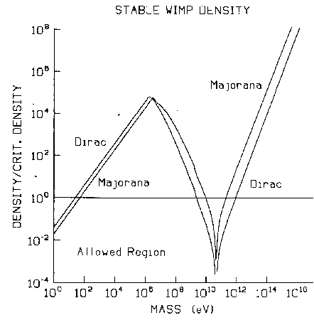
Fig. 2. Energy Density vs. Mass for Dirac and Majorana WIMPs.

If we require that the present energy density of X's is less than the present critical density^22 (rho_{c0} approx 1x10^-29 g/cm^3), then we find that there are two mass ranges of stable Dirac WIMPs allowed: m_x < 28 eV, and 2.2 GeV < m_x < 920 GeV.

Fig. 2 also demonstrates a general feature of particles annihilating in the early universe; for particles to annihilate fast enough to produce a sufficiently small energy density, the annihilation rate must be large. For masses above T_dec, the final energy density varies roughly as one over the cross section, and, as we might expect, the dip in the graph around 90.0 GeV corresponds to the peak of the annihilation cross section.

Having calculated the final energy densities of Dirac WIMPs, one might expect that a similar result could be obtained for Majorana WIMPs by simply reducing the number of degrees of freedom by a factor 2, unfortunately however, as was originally pointed out by Goldberg [12] for photinos, the annihilation cross section for non-relativistic Majorana particles is momentum dependent. Since the procedure for calculating such a cross section is slightly unusual, it may be worthwhile to go through some of the highlights of the non- relativistic calculation. Following Haber and Kane [13], we simply write down a standard Feynman diagram (fig. 3) where the directions of the arrows on the X lines are arbitrary. Now, since the X and anti-X particles are identical fermions, we must anti-symmetrize under exchange, which means subtracting the amplitude for a diagram with the roles of the incoming particles interchanged.

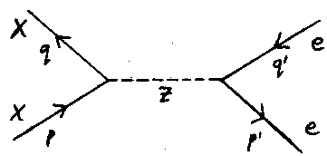
Fig. 3. Feynman diagram for X anti-X annihilation.

To make things a little easier, however, we can simply anti-symmetrize the vertex first. Writing the vertex factor as A, we have:

A = const.( vbar(q,s') gamma^µ (1 - gamma^5) u(p,s) - vbar (p,s)gamma^µ (1 - gamma^5) u(q,s')). (2.34)

But, using the identities

u (k,s) = C vbar^T(k,s) , (2.35)

v (k,s) = C ubar^T(k,s) , (2.36)

u^T(q,s')C gamma^µ (1 - gamma^5)u (p,s) = (u^T(q,s')C gamma^µ (1 - gamma^5)u (p,s))^T (2.37a)

= u^T(p,s)C gamma^µ (1 + gamma^5)u (q,s') , (2.37b)

where C is the charge conjugation matrix, we find

A = const. ( 2 vbar (p,s) gamma^µ gamma^5 u (q,s') . (2.38)

Thus, there is effectively only an axial vector coupling for Majorana annihilation. We can now write the invariant amplitude for the case M_z ť m_x as

= (g^2/4 M_z^2 cos^2theta_w)vbar(p,s)gamma^µ gamma^5u(q,s')g_{µ nu}vbar_e(q',S')gamma^nu(C_V-C_A gamma^5)ue(p',S) (2.39)

Using the usual spin-sum and trace techniques we find, neglecting the electron mass^44, that the unpolarized square of the invariant amplitude is:

= g^4/(16 M_z cos^4theta_w)2(C_V^2 + C_A^2)(2 m_x^4 - 2 m_x^2(t+u) + u^2 + t^2 - 2s), (2.40)

where s, t, and u are the usual Mandelstam variables. Hence in the limit that the x particles are non-relativistic we find, in the center of mass frame

dsigma/d_Omega = (G_F^2/4 pi^2 v) (C_V^2 + C_A^2) |p|^2 (1 + cos^2theta) , (2.41)

or

sigma = (G_F^2/3 pi v) 4 (C_V^2 + C_A^2) |p|^2 . (2.42)

By analogy to quantum mechanics, this momentum dependence is refered to as a p-wave suppression.

Krauss [14] gives <|p|^2> = (3/2) m_x kT, so we can write

< sigmav> _M = (G_F^2/2 pi) m_x^2 N_A (kT/m_x) = < sigmav> _D x , (2.43)

where subscripts M and D indicate Majorana and Dirac respectively.

Given this change in the cross section we can repeat the freeze-out calculations for Majorana WIMPs; eq.s (2.15), (2.18), (2.19), and (2.21) to (2.24) become:

d f/dx = b x (f^2 - f_eq^2) (2.44)

d f_eq/dx = bx_f f_eq^2 , at x_f = k T_f / m_x . (2.45)

d f/dx = b x f^2 , x < x_f . (2.46)

exp (1/x_f) (x_f^(-3/2) - (3 /2)x_f^(1/2) ) = 2 b k^3/(2 pi)^3/2 (2.47)

f(x_f) _1 f_eq(x_f) approx 1/(bx_f^3) . (2.48)

f(x) = 2/(b 2 x_f^3 + b (x_f^2 - x^2) ) . (2.49)

f(0) = 2/b( 2x_f^3 + x_f^2 ) . (2.50)

Also, since Majorana particles are their own anti-particles, they have only half as many degrees of freedom as Dirac particles, so eq.(2.33) becomes

rho = m_x n_0 = m_x f(0) (4/11 ) T_gamma0^3 . (2.51)

The numerical results for Majorana particles are also shown in fig. 2. As was to be expected, the suppression of the cross section increases the final energy density of Majorana particles over that of Dirac particles. Using our previous value for the critical density^33, we find the allowed mass ranges for stable Majorana WIMPs to be: m_x < 55 eV, and 9.5 GeV < m_x < 200 GeV.

3. Hidden Sectors

At present, there are various theories which predict new exotic particles, which are, as yet, unobserved. In some theories this non-observance is explained by the fact that these hypothetical particles interact with ordinary matter only through the gravitational force. This excludes the possibility that these particles can be produced in present-day accelerators, hence the name hidden sectors. Any lab set up to detect some effect of these hidden particles would require extraordinarily high energies and densities. Of course the one lab that fits the bill is the early Universe. Presumably, at some very early time these hidden particles were in a thermal equilibrium with normal matter, and they effectively decoupled when gravitational interactions became unimportant on the quantum scale^23. The various exotic particles will remain in a thermal equilibrium of their own, and different exotic species will drop out of equilibrium when the temperature drops below their mass. In this scenario, if a certain species of particles is stable, and we know their cross section for annihilation, we can go through the same type of freeze-out calculation as in the last section, and find, for a given mass, the resulting energy density. Alternatively, if we assume a cross-section of the form^24

< sigmav> = alpha^2/m^2 (3.1)

where alpha is a dimensionless factor, then for a given mass we can calculate the value of alpha, alpha = alpha_c(m), such that the energy density of the species of hidden particles equals the critical density. Since we have found that the energy density varies as 1/ < sigmav> , alpha_c is a minimum allowed value: for a given mass, values of alpha smaller than alpha_c will produce an energy density greater than the critical density. A plot of alpha_c vs. m is given in fig. 4. For large values of m, alpha becomes incredibly large, so if hidden sectors exist with stable particles having such large masses, they must experience very strong interactions. An alternative way to interpret this result is that for a given value of alpha, there is a definite mass m, which is an upper bound on the masses of stable particles which annihilate with the cross-section given by eq. (3.1). For interactions that correspond in strength to the strong interactions, ie. alpha approx 1, the upper bound on stable masses is roughly 100 TeV, and for interactions that correspond in strength to the electroweak interactions, ie. alpha approx 1/137, the upper bound is roughly 1 TeV. It should be noted that these limits will apply to the lightest particle with a particular conserved quantum number, since such a particle must be stable.

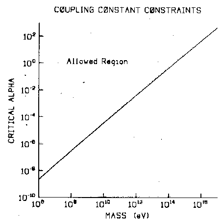
Fig. 4. Critical coupling constant vs. Mass.

For the special case that the particle under consideration is the lightest particle in the sector, then this particle will have no channels that it can annihilate into, so, the number of these particle per comoving volume must stay at its equilibrium value. The resulting upper bound on the mass in this case would be in the eV to hundreds of eV range.

4. Unstable Weakly Interacting Massive Particles

We now turn to the case of WIMPs which decay into "invisible"^25 ultra-relativistic particles. If the energy density of the WIMPs ever dominates over that of other particles, it will affect the evolution of the Universe. The amount of time it takes the X's to decay, and the amount of time it takes for its decay products to red-shift away, will determine when and for how long the Universe is matter or radiation dominated. Not only does a radiation dominated Universe expand at a different rate from a matter dominated universe, but density perturbations can only grow^26 in a matter dominated universe. For these reasons limits can be placed on lifetimes for a given initial^27 energy density for X.

At this point it would be useful to note the difference between the evolution of ultra- relativistic and non-relativistic energy densities. Since lengths grow like R(t), number densities are proportional to R(t)^(-3). Since the energy of a non-relativistic particle is approximately m, we have

rho_{NR} = m const./R^3 . (4.1)

The energy of an ultra-relativistic particle is equal to its momentum, which is proportional^28 to 1/R(t), so^29 rho_R = const./R^4 . (4.2)

With the Universe starting as an ultra-relativistic gas, the energy density goes as R^-4. Eventually, however, as the temperature drops, some particles become non-relativistic and their energy density will vary as R^-3 which must, at some point, become larger than the energy density of the radiation (or ultra-relativistic particles). At this point the Universe goes from being radiation dominated to matter dominated. If the largest contribution to the matter energy density is from the X particles, which subsequently decay into relativistic daughter particles (P's), then there is a second radiation dominated era. Finally the energy density of the other non-relativistic particles catches up, and there is a final matter dominated era. This series of events is depicted in fig. 5.

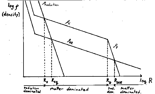
Fig. 5. Energy density vs. Cosmic Scale Factor.

It should be noted that the approximation that all the X particles decay simultaneously has, and will be, made in this discussion. It has been shown^30 that this sudden decay approximation leads to a 10%-20% error in the final results.

It can be seen from fig. 5 that if the X decay occurs before R = R_x, or if rho_x < rho_{NR}, then neither X nor its decay products significantly affects the development of the Universe. The constraint that X and its decay products P do not affect the evolution of the Universe at all, due to the above stated reasons, results^31 in lower upper bounds on possible lifetimes than will be discussed here.

We can write the energy density of the X particles before decay as

rho_x = m_x eta_x n_gamma (4.3)

where eta_x is the ratio of the number density of X particles to the number density of photons n_gamma. If we normalize the cosmic scale factor so that at the present time R(t_0) = R_0 = 1 ( a subscript 0 will indicate the present value throughout), then

n_gamma = n_gamma0 /R^3 , (4.4)

and n_gamma0 can be determined from eq (1.25). Using T_gamma0 = 2.7 K, we find that n_gamma0 _1 399/cm^3, so, rho_x becomes

rho_x = m_x eta_x n_gamma0 /R^3 . (4.5)

When the X particles decay at t = t_D, R = R_D, their energy goes into their relativistic decay products, the P's, which have an energy density given by

rho_p = rho_{c0} Omega_p / R^4 , (4.6)

where Omega represents the ratio of present energy density of a given type of particle to the present critical energy density

rho_{c0} = 3 H_0^2 / (8 pi G ) . (4.7)

Since rho_p = rho_x at R = R_D, we have

R_D = rho_{c0} Omega_p / (m_x eta_x n_gamma0 ) . (4.8)

If we now compare the energy density of X's to other non-relatvistic particles, we find

x = rho_x /rho_{NR} = m_x eta_x n_gamma0 / (rho_{c0} Omega_NR) = Omega_p / Omega_{NR} R_D . (4.9)

As mentioned previously, if x < 1, then the X and P energy densities are never dominant. However, for x > 1, provided that they do not decay too early, the X's, and later the P's, do dominate. In fact, if the energy density of the other non-relativistic particles becomes equal to the energy density of the background radiation^32 at R = R_eq, then the X's begin to dominate at an earlier time corresponding to

R_x = R_eq / x . (4.10)

The X domination will continue until R = R_D, then the P's will dominate until the non- relativistic particles take over when rho_{NR} = rho_p at R_{NR}, which is given by

R_{NR} = Omega_p / Omega_{NR} = x R_D . (4.11)

To get a constraint on the lifetime of the X particle, we need a relation between time and the energy density. Following Steigman and Turner [1], we make the rough approximation^33 that during the X domination

6 pi G rho_x t^2 approx 1 . (4.12)

So, the time of X decay is given by

t_D = R_D^(3/2) /(6piG m_x eta_x n_gamma0)^(1/2) . (4.13)

To obtain the appropriate constraints, we must consider several different scenarios of X decay; the simplest of these scenarios is that the X's have not yet decayed, ie. R_0 < R_D. In this case we would require that the present energy density of the X's is less than the present critical density, so , from eq.s (4.5) and (4.7), we have

m_x eta_x < 3 H_0^2 / (8 pi G n_gamma0) approx 15 eV . (4.14)

The next case to be considered is that the X's have decayed, and that their ultra-relativistic decay products provide the dominant energy density, ie. R_D < R_0 < R_{NR}. If the P's are sufficiently interactionless, then this possibility cannot be ruled out at present. Again, we make the requirement that the present energy density of P's is less than rho_{c0}, which, from eq.s (4.8) and (4.13), gives

t_D < 3 H_0^2 /(32(pi G n_gamma0 m_x eta_x)^2) (4.15a)

< 1.9 x 10^12 (eV)^2 yrs / (m_x eta_x)^2 . (4.15b)

Examining the previous inequality, we note that for larger values of m_x eta_x, the time of decay t_D must occur earlier, which means that the era in which density perturbations can grow is moved further back in the history of the Universe, and at some point this will conflict with our ideas of galaxy formation. To explain why this is so, we must present a brief survey of what these ideas are^31.

To explain the observed clustering of matter in our Universe, it is supposed that these large density variations grew out of small density perturbations that were present quite early in the evolution of the Universe. It proves convenient to describe density perturbations by the spectrum of density contrasts^34 (delta rho/rho) over various length scales, and to represent a given length scale by a comoving^35 length, or, as it is more commonly called, by a comoving wavelength lambda. Any comoving wavelength lambda is related to a proper^36 wavelength , lambda_prop, at the present time by lambda = lambda_prop/R. It is useful to describe the initial spectrum^37 of density contrasts by (delta rho/rho)_H (lambda), the value of a density contrast on a given length scale lambda when that scale entered the horizon, that is when lambda_prop = ct. Now, density perturbations not only lead to matter clumping, but they also produce anisotropies in the microwave background radiation; Steigman and Turner [1] require that (delta rho/rho)_H be less than roughly 10^-3 to 10^-4 for consistency with the measured isotropy of the microwave background radiation.

As suggested previously, linear density perturbations (ie. delta rho/rho « 1) grow proportional to R(t) during matter dominated eras, but do not grow during radiation dominated eras. At some point R will have increased so much that the density perturbations enter the non-linear regime (ie. delta rho/rho _1 1). Steigman and Turner [1] claim that studies of galaxy-galaxy correlations indicate that the scale^38 lambda_nl = 5 h_0^-1 Mpc is going non-linear at the present time (where h_0 is determined by H_0 = 100 h_0 km/Mpc s).

We now have a condition for the observed gravitational clustering to occur: during matter dominated eras density contrasts on the scale lambda_nl must grow by a factor approx 10^3 to 10^4 between the time lambda_nl enters the horizon, and the present. Assuming that R_{NR} < R_0 = 1, the total growth factor for density perturbations since the beginning of X domination is given by

gamma = (R_D/R_x) (R_0/R_{NR}) = 1/R_eq . (4.16)

It should be noted that gamma is independent of any properties of the X's or P's, and has the same value whether of not the X particles exist at all; this can be seen in fig. 5. For the case R_{NR} > R_0 = 1, gamma becomes

gamma = R_D/R_x = R_{NR}/R_eq , (4.17)

which will actually be slightly larger than the value given in eq. (4.16). To find the value of R_eq, we must have the energy density of the background radiation

rho_{BR} = rho_gamma0 A / R^4 , (4.18)

where rho_gamma0 is determined from eq. (2.6), and A is given by^39

A = 1 + (7/8) (T_nu / T_gamma)^4 N_nu = 1 + (7/8)(4/11)^4/3 N_nu , (4.19)

where N_nu is the number of species of 2-component relativistic neutrinos or WIMPs at the time in question. Now, R_eq can easily be solved for giving

gamma = 1/R_eq = 3 Omega_{NR} H_0^2 / 8 pi G rho_gamma0 A . (4.20)

For Omega_{NR} approx 0.2, gamma approx 4 x 10^3, which is about the factor of growth needed, but density contrasts on all scales cannot grow by this factor. It is plausibly assumed that clumping on a given length scale cannot occur until that scale has entered the horizon (in other words, two particles can not attract each other gravitationally until they are inside each other's light cones). This means that since larger scales enter the horizon at later times, density contrast for scales above a certain value (ie. that enter the horizon after X domination has begun) will undergo less growth than is given by eq. (4.16). If a scale enters the horizon at R = R_1, then the growth that the density contrast on this scale undergoes is gamma_1 = gamma(R_x/R_1), or since lambda = t/R proportional to R^(1/2),

gamma_1 = gamma (lambda_x / lambda_1 )^2 . (4.21)

Using eq.s (4.5) and (4.18) we find that

R_x = rho_gamma0 A / (m_x eta_x n_gamma0) , (4.22)

so, with eq. (4.13)

lambda_x = (rho_gamma0 A/6piG)^(1/2) /(m_x eta_x n_gamma0) (4.23a)

approx 257.9 A^(1/2) eV Mpc/m_x eta_x . (4.23b)

From this equation we can see that gamma_1 is independent of A.

To ensure that enough growth of density contrasts occurs at appropriate scales to account for the presently observed clumping, we can require that X domination occurs late enough so that density contrasts on the scale lambda_nl = 5 h_0^-1 Mpc grow by a factor of roughly 10^3. This means that lambda_x > lambda_nl/2, or^40

m_x eta_x < 100 h_0 A^(1/2) eV approx 90 eV . (4.24)

The last scenario of X decay to be considered is that the decay occurs so early that density contrasts can grow sufficiently in the second matter dominated era. This will be the case if R_{NR} < 10^-3, that is the energy density of the non-relativistic matter surpasses the P energy density soon after the X energy density passes the background radiation energy density, or, to phrase it in a different manner, the X's decay soon after becoming dominant. This constraint implies that^41 x R_D = R_{NR} < 10^-3, that is

R_D < 10^-3 rho_{c0} Omega_{NR} / m_xeta_x n_gamma0 , (4.25)

or^42,

t_D < (3/32) (10^-3 Omega_{NR} H_0^2)^(3/2) /(pi G n_gamma0 m_x eta_x )^2 (4.26a)

< 1.8 x 10^7 (eV)^2 yrs / (m_x eta_x )^2 (4.26b)

Using the results above, we can easily obtain maximum lifetimes for masses less than about 3 MeV, by noting that in this mass range^43, eta_x = ^3/11 for Majorana particles, and eta_x = 6/11 for Dirac particles. However, for WIMPs with masses above 3 MeV, we shall need the densities calculated in section 2.

A plot of maximum lifetime vs. mass for Majorana particles is shown is fig. 6. It can be seen, or calculated from eq. (4.26b), that a WIMP with a mass of 17 keV, corresponding to the so-called "Simpson's neutrino", has an upper bound on its lifetime of about one year.

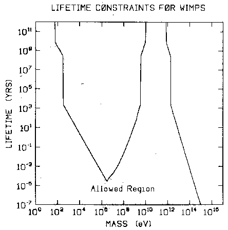
Fig. 6. Lifetime constaints for Majorana WIMPs.

5. Conclusion

Although we have given a single set of limits for Dirac and Majorana WIMPs above , due to the uncertainty in the actual value of the critical density, these cannot be taken as exact limits. The present critical density is thought^33 to be between 4.67 x 10^-30 g/cm^3 and 1.88 x 10^-29 g/cm^3; the present energy density of the Universe is also not known exactly, but it is thought to be between 0.1 rho_{c0} and 2 rho_{c0}. If the present energy density is larger (smaller) than the critical density, then the allowed energy density of WIMPs is larger (smaller) as well. Thus, these experimental uncertainties preclude final, exact limits on WIMP masses, one can only give order of magnitude estimates.

The same kind of uncertainties apply to our analysis of Hidden Sectors, and, in addition, we cannot determine exactly the amount of heating (due to the annihilation of particles with masses below 10^19 GeV) that the photon gas has undergone since the time these particles are thought to have been in equilibrium with ordinary matter. As well, the discussion of the growth of density perturbations is greatly simplified, and necessarily so, since there is, as Peebles [11] points out, "a broad range of ideas on the origins of galaxies and clusters of galaxies because it proves easy to invent detailed scenarios and so difficult to put them to the test."

Hence, in view of the above stated uncertainties, at present the constraints calculated in this report can only regarded as rough limits.

Footnotes

1. Or an infinite number of singularities.

2. By stable we mean a lifetime greater than the age of the Universe, ie. tau > 10^10 years.

3. This follows the nomenclature of Steigman and Turner [1].

4. For a thorough review of Cosmology see Weinberg [2].

5. When discussing temperatures in the early Universe it is often useful to use eV rather than Kelvin, so that temperatures can compared directly to energies or masses. The temperature in Kelvin can be found by dividing by k, Boltzmann's constant.

6. If the X particles were charged, then photons could also produce X's and anti-X's through pair production.

7. Since Majarona particles are their own antiparticles, if X were a Majorana particle, then the number density of anti-X particles would be the number density of X particles.

8. In the early Universe, assuming positive or negative curvature makes little difference, see appendix A.

9. Where a is Stephan's constant. For a more detailed discussion of this equation see appendix B.

10. See appendix B.

11. See ref. [3].

12. Kolb and Turner [4] give N_A = _1 (C_v^2 + C_A^2)i , where the sum is over particles with masses less than m_x, and where C_v = T_3 - 2 Q sin^2 theta_w , and C_A = T_3, where T_3 is the 3 component of weak isospin, Q is the charge, and theta_w is the Weinberg angle. For calculational purposes we use Lee and Weinberg's [3] value of N_A = 14.

13. This includes a Breit-Wigner resonance, which accounts for the fact that when the center of mass energy is greater than M_z, real Z's can be produced, which subsequently decay. See ref [5]. For calculational purposes Gamma_z = 8.0 GeV was used.

14. See appendix B.

15. Here N_f = 12, this includes e^-, nu_e, nu_µ , X, and their antiparticles, assuming the X's are Dirac particles.

16. c.f. eq. (2.3)

17. The decoupling temperature used in fig. 2 was adjusted to obtain a smooth transition from the region m < T_dec to the region m > T_dec.

18. This factor must be even smaller for freezing temperatures above 100 MeV to take into account the annihilation of µ ^+µ ^-, pi^+pi^-, etc.

19. See ref. [2]

20. Due to severe technical difficulties, the present neutrino temperature has not been measured. For a thorough discussion of the measurement of T_gamma0 see refs. [2] and [6].

21. See eq.s (2.16) and (2.11)

22. The critical density is the density corresponding to a flat Universe, that is, a Universe which is just balanced between collapse and continual expansion. See appendix A.

23. That is when the temperature dropped below the Planck mass, Mp = 1/G^(1/2) = 1.22 x 10 ^19 GeV. We will assume that since this decoupling, the number of degrees of freedom in the ultra-relatvistic gas has decreased by a factor of 100.

24. For a renormalizable theory, and so as to not violate Unitarity, we expect this type of form for a cross section, at least at high energies. Unless of course there is a p-wave supression, as for Majorana particles.

25. ie. particles that interact with ordinary matter at most weakly or gravitationally.

26. See Mezaros [7].

27. That is the density after any annihilation is finnished.

28. See eq. (2.1)

29. Eq. (4.1) and (4.2) can also be obtained by putting the appropriate equation of state into the the conservation of energy eq. See appendix A.

30. See Turner [8].

31. See Steigman and Turner [1].

32. That is the energy density of photons and neutrinos or WIMPs with masses less than 1.6 x 10^-4 eV.

33. See appendix A.

34. The density contrast is actually related to the fourier component of delta rho/rho. See ref. [1]

35. A comoving length is a length measured with comoving coordinates. Comoving coordinates are defined so that fundamental points (points which follow the expansion of space-time) have constant values as their coordinates. See Weinberg [2].

36. That is the wavelength actually measured by an observer with "rods" and "clocks". 37. Inflationary models predict a Zeldovich spectrum: (delta rho/rho) = const. lambda^0 = constant, however this spectrum is thought to be reasonable for other reasons as well, that is, it is the only scale-invariant (power-law) spectrum that does not blow-up at either large or small scales. See Primack [10].

38. The scale 1 Mpc corresponds roughly to a galctic size perturbation.

39. The factor of 7/8 accounts for Fermi-Dirac statistics, and the factor 4/11 accounts for the e^+e^- heating of the photon gas. See appendix B.

40. Assuming A = 1.45, h_0 = 0.75.

41. For this condition to apply it is also neccesary that R_eq < 10^-3. This means that, from eq. (3.20)

R_eq = rho_gamma0 A / rho_{NR} rho_{c0} , or Omega_{NR} h_0 > 0.024 A.

If R_eq > 10^-3, then the required amount of growth would not have occured, even without any X's present at all, that is, we can conclude that since galaxies and clusters did form, our ideas about the formation of large scale structure are in error.

42. In deference to Steigman and Turner [1] we have taken Omega_{NR} h_0 < 0.25; to be consistent with our previous choice of h_0 = 0.75, Omega_{NR} must be Omega_{NR} < 0.45. See appendix A.

43. A factor of 3/4 for Fermi-Dirac statistics, 4/11 for e^+e^- heating, and a factor of 2 for Dirac particles, since they have twice as many degrees of freedom (ie. particle and antiparticle). See appendix B.

44. When the outgoing particle mass is almost equal to the X mass, there is a slight rise in the cross section that we will not consider here. See [14].

Appendix A: Cosmology

The most general metric for an isotropic homogeneous universe is the Robertson- Walker metric^4

ds^2 = - dt^2 + R(t)^2 (dr^2/(1- kr^2) + r^2 dtheta^2 + r^2 sin^2theta dphi^2) . (A.1)

Combining this with the Einstein equations (using the energy momentum tensor of a perfect fluid) gives an equation for the scale factor R(t),

Rdot^2 = (8/3) pi G rho R^2 - k . (A.2)

where we have assumed that the cosmological constant _1 is zero here. We also have an equation for energy conservation,

pdot R^3 = d/dt ( R^3 (rho + p) ) , (A.3)

or d/dR ( rho R^3 ) = - 3 p R^2 . (A.4)

where p is the pressure, and rho the energy density. Given an equation of state p = p(rho), we can solve for rho(R). If p = a rho, we find

rho proportional to R^(-3(1 + a)) . (A.5)

For non-relativistic particles a approx 0, while for ultra-reletvistic particles a = ^1/3. Rewriting eq. (A.2) we can find the present energy density of the Universe

rho_1 = (3/8 pi G) ( H_0^2 + k/R_0^2) , (A.6)

where H is Hubble's parameter, Rdot/R, and subscripts _0 indicate the present value, as throughout. It can easily be seen that the curvature parameter k is positive or negative depending on whether rho_0 is greater or less than the critical density

rho_{c0} = 3 H_0^2/8 piG . (A.7)

For rho_0 > rho_{c0}, the Universe is closed and eventually contracts, while for rho_1 < rho_{c0} the Universe is open and expands forever. It should be noted that there is a large uncertainty associated with the values of rho_0 and H_0. The ratio Omega = rho_0/rho_{c0} is thought to have a value between 0.1 and 2, although the contribution due to baryons is measured to be only Omega_B approx 0.01. If we write H_0 as H_0 = 100 h_0 km/Mpc s, then the present limits on Hubble's parameter are 0.5 < h_0 < 1. However, large values of both Omega and h_0 would require that the Universe to be quite young. Steigman and Turner [1] give a lower bound on the age of the Universe of 1.0 -1.3 x 10^10 years, which, along with h_0 > 0.5, implies that

Omega h_0^2 < 0.25 - 0.75 . (A.8)

In this report, for calculational purposes we use the value h_0 = 0.75.

When considering the early Universe, it is common to set k = 0, which gives a flat Universe with rho = rho_c. Weinberg [2] gives a numerical comparision of the second and third terms in eq. (A.2), and shows that the curvature term k has been insignificant up to the present time. Here we will be satisfied with a hand-waving argument due to Primack [10]. One may recall that on 2-dimensional surface, curvature effects are proportional to the area of the portion of the surface being examined; in the early Universe, the volume that we can examine is limited by the horizon, so at early enough times curvature will be insignificant.

To find an equation giving the age of the Universe as a function of R during the X domination, we note that during this period the energy density was proportional to R^-3, so from eq. (A.2)

rhodot_x/rho_x = - 3 Rdot/R = - 3 (8 pi G rho_x / 3)^(1/2) . (A.9)

Which yields, upon integration

t = 1/(6 pi G rho_x)^(1/2) + C_1 . (A.10)

It can be shown that C_1 is less than tx (the time of X domination) by roughly an order of magnitude, so, for tx < t < t_D (the time of X decay) we have

6 pi G rho_x t^2 approx 1 . (A.11)

Appendix B: Statistical Mechanics

The basic idea that we need to use from Statistical Mechanics is that particles with integral spin (bosons) obey Bose-Einstein statistics, and thus have distribution function (which gives the probability that a state of energy E is occupied) given by

b(E) = 1/(exp((E - µ )/kT) - 1) , (B.1)

and particles with half-integral spin (fermions) obey Fermi-Dirac statistics, and have a distribution function given by

f(E) = 1/(exp((E - µ )/kT) + 1) , (B.2)

where k is Boltzmann's constant, T is the temperature, and µ is the chemical potential. For most presently observed particles, µ « kT, so it can safely be ignored. There is some uncertainty as to whether this is actually true for neutrinos; Weinberg [2] gives an experimental limit of

| µ _{nu_e} | < 60 eV . (B.3)

We will assume that µ _1 0 for all particles. However, if a particle has a chemical potential µ , then its antiparticle must have a chemical potential -µ , so for photons and non- relativistic Majorana particles, the chemical potential is identically zero.

Given eq.s (B.1) and (B.2) we can find the number density of bosons and fermions by integrating over momentum space and dividing by (2pih)^3 (following past practice, we will set h = c = 1). We find

N_B = ( g_s/(2pi)^3) int d^3p (exp((p^2 + m^2)^(1/2)/kT) - 1)^-1 , (B.4a)

= ( g_s/(2pi)^3) int_0^infinity 4pi p^2 dp (exp((p^2 + m^2)^(1/2)/kT) - 1)^-1 , (B.4b)

= ( g_s/2pi^2) int_0^infinity dp p^2 (exp((p^2 + m^2)^(1/2)/kT) - 1)^-1 . (B.4c)

Similarily,

N_f = ( g_s/2pi^2) int_0^infinity dp p^2 (exp((p^2 + m^2)^(1/2)/kT) + 1)^-1 , (B.5)

where g_s is the number of internal degrees of freedom. For example, a spin 1/2 Dirac particles has 4 degrees of freedom, since a Dirac spinor is a four component object, with 2 degrees of freedom to account for particle and antiparticle, which is then multiplied by 2, since the particle and antiparticle have 2 spin states each. Spin 1/2 Majorana particles have 2 degrees of freedom; they can be represented by Dirac spinors, but only two of the components are independent. They have 2 spin states, but they are their own antiparticles. Photons are spin-1 particles, but only have 2 spin states since they are massless. They are also their own antiparticle, so they have only 2 degrees of freedom as well.

Since the approximate solution for non-relativistic fermions is given in eq. (2.20), we will concentrate on relativistic particles here, and thereby uncover the "mysterious" factors of 3/4 and 7/8. For p_1 ť m, we have

N_b = ( g_s/2pi^2) int_0^infinity dp p^2 (exp( p /kT) - 1)^-1 , (B.6)

and

N_f = ( g_s/2pi^2) int_0^infinity dp p^2 (exp( p /kT) + 1)^-1 . (B.7)

Gradshteyn and Ryzhik [9] give the following results:

int_0^infinity dx x^(nu-1) / (e^(ax) - 1) = a^-nu Gamma(nu) zeta(nu) , (B.8)

and

int_0^infinity dx x^(nu-1) / (e^(ax) + 1) = ( 1 - 2^(1-nu)) a^-nu Gamma(nu) zeta(nu) , (B.9)

where Gamma(nu) is the Gamma Function, Gamma(n) = (n - 1)! , and zeta(nu) is the famous Riemann Zeta function

zeta(nu) = Sum_{k=1}^infinity k^-nu . (B.10)

So,

N_b = (g_s/pi^2) zeta(3) (kT)^3 , (B.11)

N_f = (3/4) (g_s/pi^2) zeta(3) (kT)^3 . (B.12)

Similar results can be found for the energy densities

rho_b = ( g_s/2 pi^2) int_0^infinity dp p^3 (exp( p /kT) - 1)^-1 , (B.13a)

= ( g_s pi^2 /30) (kT)^4 . (B.13b)

rho_f = ( g_s/2 pi^2) int_0^infinity dp p^3 (exp( p /kT) + 1)^-1 , (B.14a)

= (7/8) ( gs pi^2 /30) (kT)^4 , (B.14b)

where we have used the fact that zeta(4) = pi^4/90. It is evident that the factors of 3/4 and 7/8 arise due to the factor (1 - 2^(1-nu)) in eq. (B.9).

Weinberg [2] gives the entropy of a gas in equilibrium (up to an additive constant) as

S(V,T) = (V/T) ( rho(T) + p(T)) , (B.15)

where p is the pressure of the gas. Since a volume V in an expanding Universe will grow like R(t)^3, we can define a quantity that is proportional to the entropy by

s equiv ( R^3/T ) ( rho(T) + p(T)) . (B.16)

For an ultra-relativistic gas, p = (1/3) rho, so s = (4 R^3/3T) rho , (B.17)

which, from eq. (2.6) gives s = (4/3) N_f a (RT)^3 . (B.18)

Now if N_f is decreased from N_f1 to N_f2 due to the annihilation of a species of particles, s will stay constant (since this is, in principle, a reversable process), so we have

(R_1 T_1)/(R_2 T_2) = (N_f2 / N_f1)^(1/3) equiv h ^(1/3) . (B.19)

For an example we take the e^+e^- annihilation. From eq. (2.7) we have for the photon e^+e^- gas N_f1 = (1/2) ( 2 + (7/8)4) = 1 + 7/4, and for the photon gas after the annihilation, N_f2 = 1, so h = 4/11 . If R is roughly constant during this process, T_1^3 = h T_2^3, or since before the annihilation T_nu = T_gamma = T_1, and afterwards T_gamma = T_2, we have, at the present time for any relativistic neutrinos or WIMPs

T_nu^3 = h T_gamma^3 = (4/11) T_gamma^3 . (B.20)

We can easily do a similar calculation for µ ^+µ ^-, pi^+pi^-, and K+K^- annihilations. Assuming that there are two types of 2-component neutrinos present in equilibrium during these annihilations (there could easily be three types, depending on the mass of nu_tau) we find h = 36/50, 50/58, and 58/66, for the µ ^+µ ^-, pi^+pi^-, and K^+K^- annihilations respectively.